Linear and non-linear: the two halves of processing

When you open a freshly stacked image for the first time, it’s almost completely black. Maybe a few bright stars, but no nebula and no galaxy, even though you know they’re in there. And then you apply a stretch and suddenly everything appears.

What happens in that step is one of the most important things to understand in astrophoto processing. The stretch divides your processing into two stages: the linear stage before it and the non-linear stage after it. Some steps only work properly in the first, others belong in the second. In my basic PixInsight workflow I already sorted the steps into these stages; here I want to explain why.

Key takeaways

• A linear image is still a measurement: every pixel value is proportional to the light that pixel collected. Twice the light, twice the value.
• The stretch makes faint things visible, by lifting the faint end of the range much more than the bright end. After it, the image is no longer proportional to the light.
• Do the “physics” in the linear stage: calibration, stacking, gradient removal, colour calibration, deconvolution and combining data from different filters or nights. They all rely on the values being proportional.
• Do the “looks” in the non-linear stage: contrast, saturation, local contrast, sharpening, star reduction and the final noise reduction, where you judge by eye.
• The stretch is a one-way street. Keep a copy of your linear image, so you can always go back.

What “linear” means

A camera sensor counts photons, or more precisely the electrons they free in each pixel. The camera turns that count into a number. Double the light and you double the number: the value is proportional to the light. That’s what linear means.

Calibration and stacking keep it that way. They subtract (darks, bias), divide (flats) and average, and none of that changes the proportionality. So your stacked image is still a measurement of the light that reached each pixel.

Then why does it look black? Because in a typical deep-sky image almost all of the data sits at the very bottom of the range. The sky background might be at 2% of full range, the faint parts of a nebula only a fraction of a percent above that. Only the cores of bright stars get anywhere near the top. On your screen 2% is a value of 5 out of 255: black. The information is all there, it’s just squeezed into the first few percent of the range.

The stretch

A stretch is a curve that maps the linear values to new ones, lifting the faint end much more than the bright end:

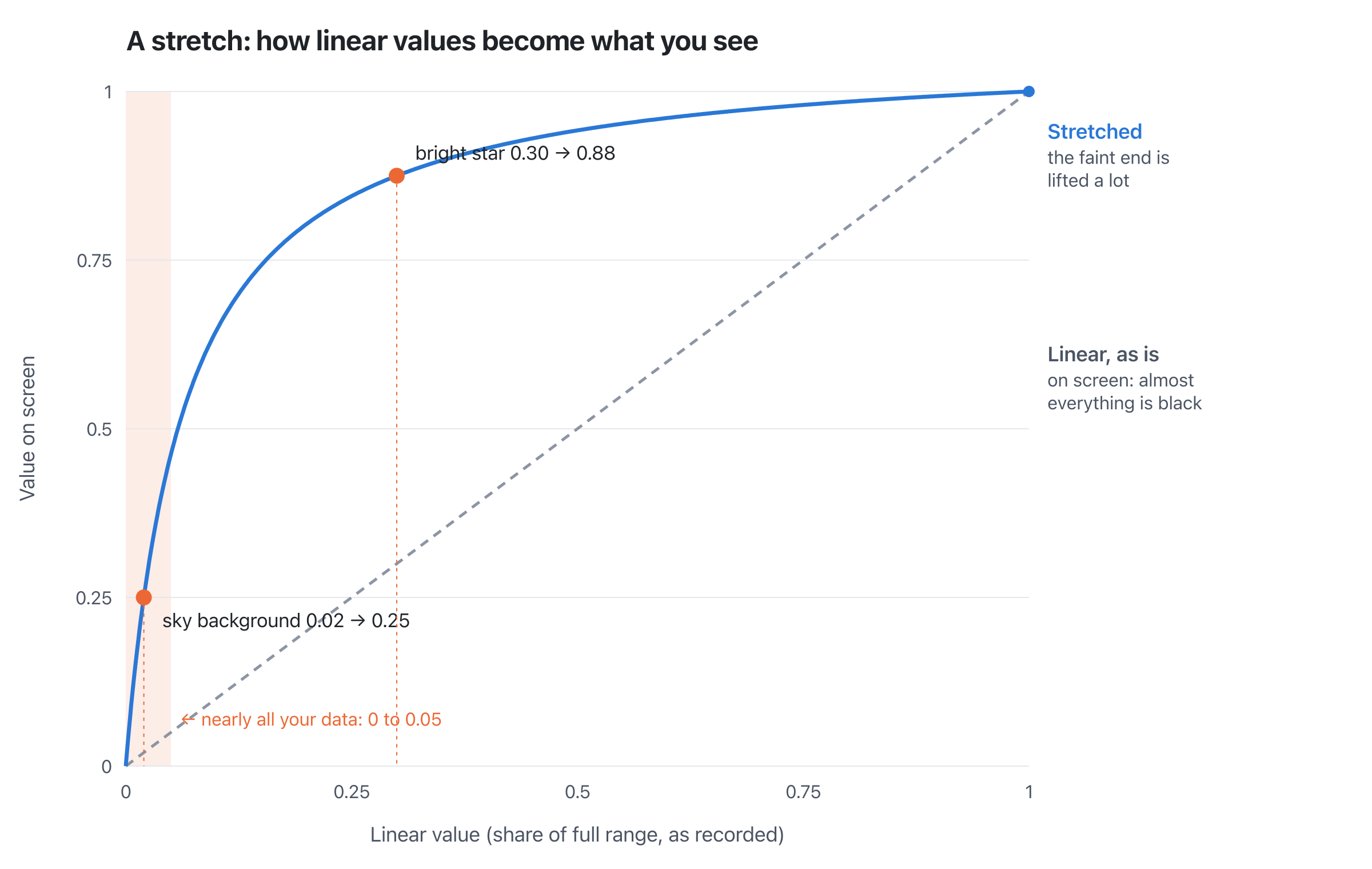
The stretch in the figure is the one PixInsight uses for its screen stretch and its HistogramTransformation, the midtones transfer function:

$$\text{MTF}(x) = \frac{(m - 1)\,x}{(2m - 1)\,x - m}$$

where $x$ is the linear value and $m$ the midtones balance (the middle slider in the histogram). With $m = 0.058$, the sky background at 0.02 ends up at 0.25, which is about where an automatic stretch puts it. A bright star at 0.30 ends up at 0.88. The faint end is lifted more than ten times, the bright end hardly at all.

That’s exactly what we want to see. But look at what it does to the numbers: values that were in a ratio of 1 to 15 (0.02 and 0.30) are now in a ratio of 1 to 3.5. After the stretch, a pixel value no longer tells you how much light there was. The image is non-linear.

Note that you don’t have to stretch to see your linear data. PixInsight’s ScreenTransferFunction (STF) and Siril’s autostretch display a stretched version on screen while the data itself stays linear. Remember that when you look at an image: what you see is not necessarily what the data is. (That’s also why an image can suddenly look white after a real stretch: the screen stretch is still applied on top.)

Why some steps need linear data

Many processing steps are based on a model of how the light got into your image. Those models describe physics, and physics is linear. Once the image is stretched, the model no longer fits.

Gradients

Light pollution and moonlight add a smooth glow to your image, usually brighter on one side. In the linear image that glow simply adds to everything: every pixel gets the same extra light as its neighbours, whether it’s background, nebula or star. So you can model the glow as a smooth surface and subtract it, and what’s left is exactly what you would have recorded without it.

After a stretch, that’s no longer true:

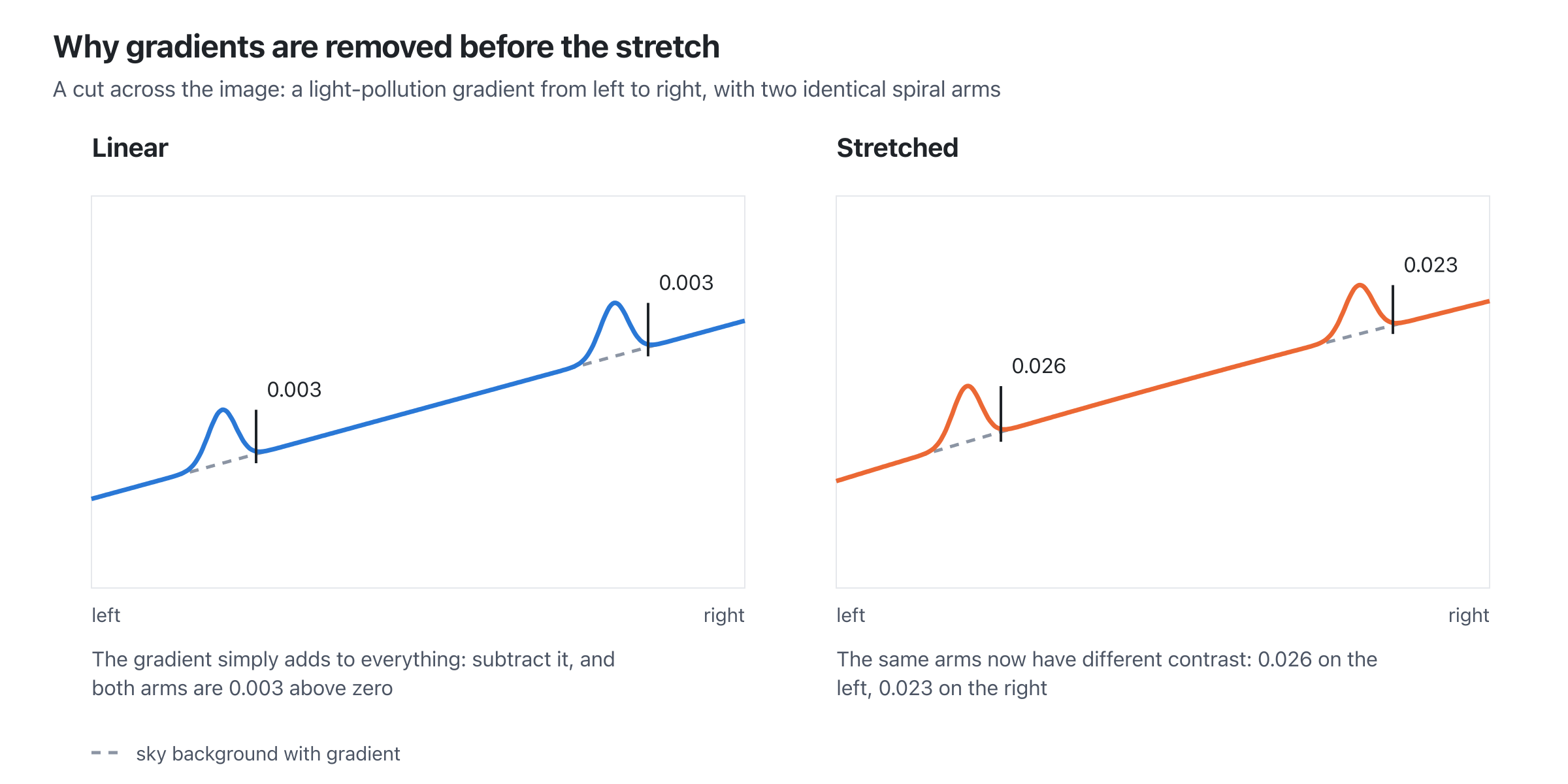
In the linear image both spiral arms add 0.003 to the background, on both sides. After the stretch, the arm on the darker left side stands out more than the one on the brighter right side, because the stretch compresses brighter values more. Subtracting a smooth background can no longer fix that: the gradient has become part of how bright your target looks. So remove gradients with DynamicBackgroundExtraction (or GradientCorrection, or Siril’s background extraction) before you stretch.

Colour

The colour of a star or a nebula is the ratio between red, green and blue. In linear data those ratios are physical: a star that’s twice as bright in red as in blue really sends twice as much red light. Colour calibration (ColorCalibration, or SPCC with star catalogue data) works by multiplying each channel by a factor until known references come out right. That only works while the ratios still mean something: in the linear stage.

A stretch can also change the colours themselves:

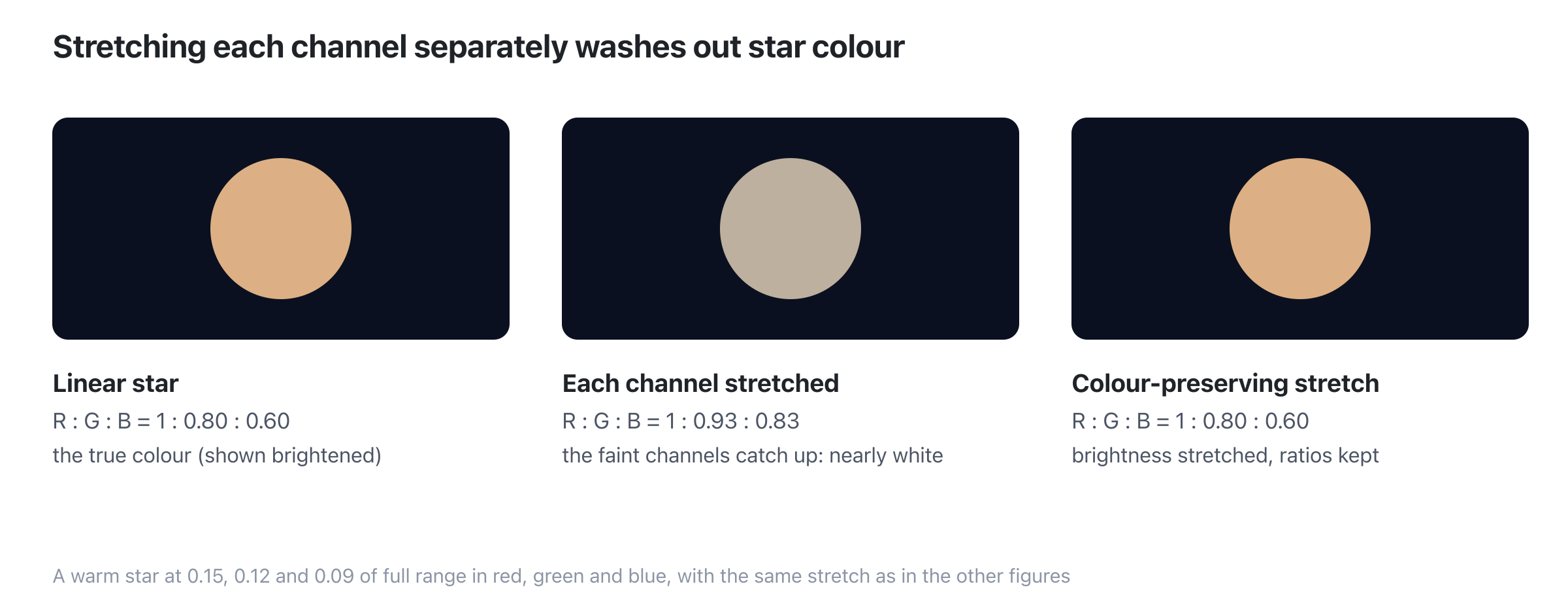
If you stretch each channel separately, the fainter channels are lifted more than the brightest one, and the ratios move towards 1. A warm, orange star becomes nearly white. That’s one reason so many astrophotos have white stars. Stretches that work on the brightness and keep the ratios (MaskedStretch, ArcsinhStretch, or HistogramTransformation applied to the lightness only) keep much more colour. That’s why I prefer them for the initial stretch.

Deconvolution

The atmosphere and your optics blur every star into a small disk: the point spread function (PSF). Mathematically that blur is a convolution: every point of light is spread out in the same way, and the results add up. Deconvolution reverses it, but only on data where light still adds up linearly. On stretched data the model is wrong, and deconvolution produces artefacts instead of detail.

Combining data

Anything that combines images relies on the values being comparable: stacking frames from different nights, building a mosaic, an HDR composition, or adding Hα from a filtered stack to a galaxy. In linear data, twice the integration time means twice the signal, and a weighted sum is a weighted sum. Once two images are stretched differently, adding them no longer means anything physical.

Noise reduction: both

Noise reduction is the exception: it can be done in both stages. In the linear stage the noise still behaves like it was recorded (its strength follows the signal), which algorithms can use. In the non-linear stage you can judge the result by eye. I usually do a gentle first pass in the linear stage, and only a very light final touch after the stretch, if any.

What belongs in the non-linear stage

Once the image is stretched, you’re working on what the viewer will see. That’s the place for everything you judge by eye:

• Contrast and brightness with curves.
• Saturation, usually with a mask to leave the background alone.
• Local contrast and dynamic range: HDRMultiscaleTransform, LocalHistogramEqualization.
• Sharpening of fine detail, with a mask.
• Star reduction, to bring your main subject forward.
• The final noise reduction, if needed.

These steps don’t depend on physics. They depend on how the image looks, and on your taste. In the linear stage you’d be doing them half blind, through a screen stretch that changes as the data changes.

Masks also work best here. A mask made from the stretched image follows what you see: the brightness of the nebula, the stars, the background. In the linear stage almost everything is near black, so a brightness mask from linear data hardly separates anything.

An overview

Stage	Step	Why there
Linear	Calibration (darks, flats, bias)	Subtracting and dividing only works on values proportional to light
Linear	Stacking	Averaging and weighting frames need comparable values
Linear	Cropping the edges	So stacking artefacts don’t affect later steps
Linear	Gradient removal	Light pollution adds to everything; only in linear data can you subtract it cleanly
Linear	Colour calibration	Colour is a ratio between channels, and the ratios are only physical before the stretch
Linear	Deconvolution	The blur model (convolution) only holds for linear data
Linear	Combining data (filters, nights, mosaics, HDR)	Signals add up only in linear data
Either	Noise reduction	Linear: the noise model still holds. Non-linear: judge by eye
The stretch	MaskedStretch, ArcsinhStretch, HistogramTransformation	The one-way step between the two stages
Non-linear	Curves, contrast, saturation	You’re shaping what the viewer sees
Non-linear	Local contrast, HDR	Judged by eye, with masks
Non-linear	Sharpening, star reduction	Judged by eye, with masks

A note for smart scope users

A Seestar or Dwarf stacks your data for you and shows you a finished image. That image, and the JPEG or PNG you save from the app, is already stretched: you can’t do the linear steps on it anymore. If you want to process your data yourself, use the stacked FITS file. That one is still linear, so you can remove gradients, calibrate the colour and choose your own stretch.

Conclusion

The stretch is the turning point of your processing. Before it, you’re working with a measurement, and you correct it with steps that rely on the physics: removing what doesn’t belong (gradients), restoring what was distorted (colour, blur) and combining data. After it, you’re working with a picture, and you shape it to show what you want to show.

Keep the order, keep a linear copy, and take your time with the stretch itself. It decides how much of the work you did before it survives.